6.3.6. SubDyn Theory
This section focuses on the theory behind the BeamDyn module. The theoretical foundation, numerical tools, and some special handling in the implementation will be introduced. References will be provided in each section detailing the theories and numerical tools.
In this chapter, matrix notation is used to denote vectorial or vectorial-like quantities. For example, an underline denotes a vector \(\underline{u}\), an over bar denotes unit vector \(\bar{n}\), and a double underline denotes a tensor \(\underline{\underline{\Delta}}\). Note that sometimes the underlines only denote the dimension of the corresponding matrix.
6.3.6.1. Overview
This section focuses on the theory behind the SubDyn module.
SubDyn relies on two main engineering approaches: (1) a linear frame finite-element beam model (LFEB), and (2) a dynamics system reduction via the Craig-Bampton (C-B) method together with a static-improvement method (SIM), greatly reducing the number of modes needed to obtain an accurate solution.
There are many nonlinearities present in offshore wind substructure models, including material nonlinearity, axial shortening caused by bending, large displacements, and so on. The material nonlinearity is not considered here because most offshore multimember support structures are designed to use steel and the maximum stress is intended to be below the yield strength of the material. [DSRJ13] demonstrate that a linear finite-element method is suitable when analyzing wind turbine substructures. In this work, several wind turbine configurations that varied in base geometry, load paths, sizes, supported towers, and turbine masses were analyzed under extreme loads using nonlinear and linear models. The results revealed that the nonlinear behavior was mainly caused by the mono-tower response and had little effect on the multimember support structures. Therefore, an LFEB model for the substructure is considered appropriate for wind turbine substructures. The LFEB can accommodate different element types, including Euler-Bernoulli and Timoshenko beam elements of either constant or longitudinally tapered cross sections (Timoshenko beam elements account for shear deformation and are better suited to represent low aspect ratio beams that may be used within frames and to transfer the loads within the frame).
The large number of DOFs (~ \({10^3}\)) associated with a standard finite-element analysis of a typical multimember structure would hamper computational efficiency during wind turbine system dynamic simulations. As a result, the C-B system reduction was implemented to speed up processing time while retaining a high level of fidelity in the overall system response. The C-B reduction is used to recharacterize the substructure finite-element model into a reduced DOF model that maintains the fundamental low-frequency response modes of the structure. In the SubDyn initialization step, the large substructure physical DOFs (displacements) are reduced to a small number of modal DOFs and interface (boundary) DOFs, and during each time step, only the equations of motion of these DOFs need to be solved. SubDyn only solves the equations of motion for the modal DOFs, the motion of the interface (boundary) DOFs are either prescribed when running SubDyn in stand-alone mode or solved through equations of motion in ElastoDyn when SubDyn is coupled to FAST.
Retaining just a few DOFs may, however, lead to the exclusion of axial modes (normally of very high frequencies), which are important to capture static load effects, such as those caused by gravity and buoyancy. The so-called SIM was implemented to mitigate this problem. SIM computes two static solutions at each time step: one based on the full system stiffness matrix and one based on the C-B reduced stiffness matrix. At each time step the time-varying, C-B based, dynamic solution is superimposed on the difference between the two static solutions, which amounts to quasi-statically accounting for the contribution of those modes not directly included within the dynamic solution.
In SubDyn, the substructure is considered to be clamped, or connected via linear spring-like elements, at the bottom nodes (normally at the seabed) and rigidly connected to the TP at the substructure top nodes (interface nodes). The user can provide 6x6, equivalent stiffness and mass matrices for each of the bottom nodes to account for soil-pile interaction. As described in other sections of this document, the input file defines the substructure geometry, material properties, and constraints. Users can define: element types; full finite-element mode or C-B reduction; the number of modes to be retained in the C-B reduction; modal damping coefficients; whether to take advantage of SIM; and the number of elements for each member.
The following sections discuss the integration of SubDyn within the FAST framework, the main coordinate systems used in the module, and the theory pertaining to the LFEB, the C-B reduction, and SIM. The state-space formulations to be used in the time-domain simulation are also presented. The last section discusses the calculation of the base reaction calculation. For further details, see also [SDRJ13].
6.3.6.2. Integration with the FAST Modularization Framework
Based on a new modularization framework [Jon13], FAST joins an aerodynamics module, a hydrodynamics module, a control and electrical system (servo) module, and structural-dynamics (elastic) modules to enable coupled nonlinear aero-hydro-servo-elastic analysis of land-based and offshore wind turbines in the time domain. Fig. 6.17 shows the basic layout of the SubDyn module within the FAST modularization framework.
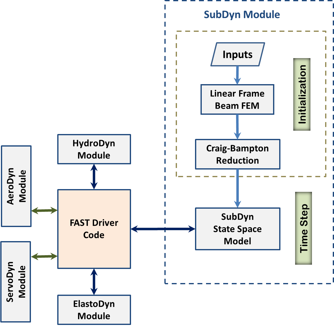
Fig. 6.17 SubDyn layout within the modularization framework
In the existing loosely coupled time-integration scheme, the glue-code transfers data at each time step. Such data includes hydrodynamic loads, substructure response, loads transmitted to the TP, and TP response among SubDyn, HydroDyn, and ElastoDyn. At the interface nodes, the TP displacement, rotation, velocity, and acceleration are inputs to SubDyn from ElastoDyn, and the reaction forces at the TP are outputs of SubDyn for input to ElastoDyn. SubDyn also outputs the substructure displacements, velocities, and accelerations for input to HydroDyn to calculate the hydrodynamic loads that become inputs for SubDyn. In addition, SubDyn can calculate the member forces, as requested by the user. Within this scheme, SubDyn tracks its states and integrates its equations through its own solver.
In a tightly coupled time-integration scheme (yet to be implemented), SubDyn sets up its own equations, but its states and those of other modules are tracked and integrated by a solver within the glue-code that is common to all of the modules.
SubDyn is implemented in a state-space formulation that forms the equation of motion of the substructure system with physical DOFs at the boundaries and modal DOFs representing all interior motions. At each time step, loads and motions are exchanged between modules through the driver code; the modal responses are calculated inside SubDyn’s state-space model; and the next time-step responses are calculated by the SubDyn integrator for loose coupling and the global system integrator for tight coupling.
6.3.6.3. Coordinate Systems
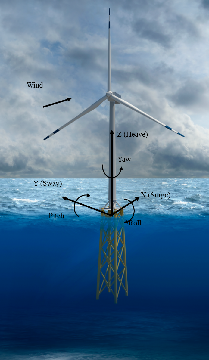
Fig. 6.18 Global (coincident with the substructure) coordinate system. Also shown are the DOFs associated with the TP reference point.
6.3.6.3.1. Global and Substructure Coordinate System: (X, Y, Z) or (\({X_{SS}, Y_{SS}, Z_{SS}}\)) (Fig. 6.18)
- The global axes are represented by the unit vectors \({\hat{I}, \hat{J}}\), and \({\hat{K}}\).
- The origin is set at the intersection between the undeflected tower centerline and the horizontal plane identified by the mean sea level (MSL) for offshore systems or ground level for land-based systems.
- The positive Z (\({Z_{SS}}\)) axis is vertical and pointing upward, opposite gravity.
- The positive X (\({X_{SS}}\)) axis is along the nominal (zero-degree) wind and wave propagation direction.
- The Y (\({Y_{SS}}\)) axis is transverse and can be found assuming a right-handed Cartesian coordinate system (directed to the left when looking in the nominal downwind direction).
6.3.6.3.2. Member or Element Local Coordinate System (\({x_e, y_e, z_e}\)) (Fig. 6.19)
- Axes are represented by the unit vectors \({\hat{i}_e, \hat{j}_e, \hat{k}_e}\).
- The origin is set at the shear center of the cross section at the start node (S,MJointID1).
- The local axis is along the elastic axis of the member, directed from the start node (S) to the end node (E,MJointID2). Nodes are ordered along the member main axis directed from start joint to end joint (per user’s input definition).
- The local axis is parallel to the global \(\text{XY}\) plane, and directed such that a positive, less than or equal to 180º rotation about it, would bring the local axis parallel to the global Z axis.
- The local axis can be found assuming a right-handed Cartesian coordinate system.

Fig. 6.19 The element coordinate system. The sketched member contains four elements, and the second element is called out with nodes S and E.
6.3.6.3.3. Local to Global Transformation
The transformation from local to global coordinate system can be expressed by the following equation:
(1)¶\[\begin{split}\begin{bmatrix} \Delta X \\ \Delta Y \\ \Delta Z \end{bmatrix} = [ \mathbf{D_c} ] \begin{bmatrix} \Delta x_e \\ \Delta y_e \\ \Delta z_e \end{bmatrix}\end{split}\]
where \(\begin{bmatrix} \Delta x_e \\ \Delta y_e \\ \Delta z_e \end{bmatrix}\) is a generic vector in the local coordinate system, and \(\begin{bmatrix} \Delta X \\ \Delta Y \\ \Delta Z \end{bmatrix}\) the same vector but in the global coordinate system; and \([ \mathbf{D_c} ]\) is the direction cosine matrix of the member axes and can be obtained as follows:
(2)¶\[\begin{split}[ \mathbf{D_c} ] = \begin{bmatrix} \frac{Y_E-Y_S}{L_{exy}} & \frac{ \left ( X_E-X_S \right) \left ( Z_E-Z_S \right)}{L_{exy} L_{e}} & \frac{X_E-X_S}{L_{e}} \\ \frac{-X_E+X_S}{L_{exy}} & \frac{ \left ( Y_E-Y_S \right) \left ( Z_E-Z_S \right)}{L_{exy} L_{e}} & \frac{Y_E-Y_S}{L_{e}} \\ 0 & \frac{ -L_{exy} }{L_{e}} & \frac{Z_E-Z_S}{L_{e}} \end{bmatrix}\end{split}\]
Where \({\left ( X_s,Y_s,Z_s \right )}\) and \({\left ( X_E,Y_E,Z_E \right )}\) are the start and end joints of the member (or nodes of the element of interest) in global coordinate system; \({L_{exy}= \sqrt{ \left ( X_E-X_S \right )^2 + \left ( Y_E-Y_S \right )^2}}\) and \({L_{e}= \sqrt{ \left ( X_E-X_S \right )^2 + \left ( Y_E-Y_S \right )^2 + \left ( Z_E-Z_S \right )^2}}\).
If \({X_E = X_S}\) and \({Z_E = Z_S}\), the \({[ \mathbf{D_c} ]}\) matrix can be found as follows:
if \({Z_E < Z_S}\) then
(3)¶\[\begin{split}[ \mathbf{D_c} ] = \begin{bmatrix} 1 & 0 & 0 \\ 0 & 1 & 0 \\ 0 & 0 & 1 \end{bmatrix}\end{split}\]
else
(4)¶\[\begin{split}[ \mathbf{D_c} ] = \begin{bmatrix} 1 & 0 & 0 \\ 0 & -1 & 0 \\ 0 & 0 & -1 \end{bmatrix}\end{split}\]
In the current SubDyn release, the transpose (global to local) of these direction cosine matrices for each member is returned in the summary file. Given the circular shape of the member cross sections, the direction cosine matrices have little importance on the member load verification. To verify joints following the standards (e.g., [ISO07][ apirp2a2014] ), however, the bending moments need to be decomposed into in-plane and out-of-plane components, where the plane is that defined by either a pair of braces (for an X-joint), or by the pair brace(s) plus leg (for a K-joint). It is therefore important to have the direction cosines of the interested members readily available to properly manipulate and transform the local shear forces and bending moments.
When member cross sections other than circular are allowed in future releases, the user will need to input cosine matrices to indicate the final orientation of the member principal axes with respect to the global reference frame.
6.3.6.4. Linear Finite-Element Beam Model
In SubDyn, the LFEB can accommodate different two-node beam element types, including Euler-Bernoulli and Timoshenko beam elements, either of constant or tapered cross sections. The tapered element formulation has been derived, but has not been implemented in the current SubDyn release.
The uniform and tapered Euler-Bernoulli beam elements are displacement-based and use third-order interpolation functions that guarantee the displacement and rotation continuity between elements. The uniform Timoshenko beam element is derived by introducing the shear deformation into the uniform Euler-Bernoulli element, so the displacements are represented by third-order interpolation functions as well.
6.3.6.4.1. Element Formulation
Following the classic Timoshenko beam theory, the generic two-node element stiffness and consistent mass matrices can be written as follows (see, for instance, [PHEL09]):
(5)¶\[\begin{split}[k_e]= \begin{bmatrix} \frac{12 E J_y} {L_e^3 \left( 1+ K_{sy} \right)} & 0 & 0 & 0 & \frac{6 E J_y}{L_e^2 \left( 1+ K_{sy} \right)} & 0 & -\frac{12 E J_y}{L_e^3 \left( 1+ K_{sy} \right)} & 0 & 0 & 0 & \frac{6 E J_y}{L_e^2 \left( 1+ K_{sy} \right)} & 0 \\ & \frac{12 E J_x}{L_e^3 \left( 1+ K_{sx} \right)} & 0 & -\frac{6 E J_x}{L_e^2 \left ( 1+ K_{sx} \right )} & 0 & 0 & 0 & -\frac{12 E J_x}{L_e^3 \left ( 1+ K_{sx} \right )} & 0 & -\frac{6 E J_x}{L_e^2 \left ( 1+ K_{sx} \right )} & 0 & 0 \\ & & \frac{E A_z}{L_e} & 0 & 0 & 0 & 0 & 0 & -\frac{E A_z}{L_e} & 0 & 0 & 0 \\ & & & \frac{\left(4 + K_{sx} \right) E J_x}{L_e \left ( 1+ K_{sx} \right )} & 0 & 0 & 0 & \frac{6 E J_x}{L_e^2 \left ( 1+ K_{sx} \right )} & 0 & \frac{\left( 2-K_{sx} \right) E J_x}{L_e \left ( 1+ K_{sx} \right )} & 0 & 0 \\ & & & & \frac{\left(4 + K_{sy} \right) E J_y}{L_e \left ( 1+ K_{sy} \right )} & 0 & -\frac{6 E J_y}{L_e^2 \left ( 1+ K_{sy} \right )} & 0 & 0 & 0 & \frac{\left( 2-K_{sy} \right) E J_y}{L_e \left ( 1+ K_{sy} \right )} & 0 \\ & & & & & \frac{G J_z}{L_e} & 0 & 0 & 0 & 0 & 0 & -\frac{G J_z}{L_e} \\ & & & & & & \frac{12 E J_y}{L_e^3 \left ( 1+ K_{sy} \right )} & 0 & 0 & 0 & -\frac{6 E J_y}{L_e^2 \left ( 1+ K_{sy} \right )} & 0 \\ & & & & & & & \frac{12 E J_x}{L_e^3 \left ( 1+ K_{sx} \right )} & 0 & \frac{6 E J_x}{L_e^2 \left ( 1+ K_{sx} \right )} & 0 & 0 \\ & & & & & & & & \frac{E A_z}{L_e} & 0 & 0 & 0 \\ & & & & & && & & \frac{\left(4 + K_{sx} \right) E J_x}{L_e \left ( 1+ K_{sx} \right )} & 0 & 0 \\ & & & & & & & & & & \frac{\left(4 + K_{sy} \right) E J_y}{L_e \left ( 1+ K_{sy} \right )} & 0 \\ & & & & & & & & & & & \frac{G J_z}{L_e} \end{bmatrix}\end{split}\]
where \(A_z\) is the element cross-section area, \(J_x, J_y, J_z\) are the area second moments of inertia with respect to principal axes of the cross section; \(L_e\) is the length of the undisplaced element from start-node to end-node; \(\rho, E, \textrm{and}\quad G\) are material density, Young’s, and Shear moduli, respectively; \(K_{sx}, K_{sy}\) are shear correction factors as shown below (they are set to zero if the E-B formulation is chosen):
where the shear areas along the local x and y (principal) axes are defined as:
and
Eq. (9) is from [SKM13] for hollow circular cross sections, with \(\mu\) denoting Poisson’s ratio.
Before assembling the global system stiffness (K) and mass (M) matrices, the individual \({[k_e]}\) and math:{[m_e]} are modified to the global coordinate system via \({[ \mathbf{D_c} ]}\) as shown in the following equations:
where m and k are element matrices in the global coordinate system.
6.3.6.4.2. Self-Weight Loads
The loads caused by self-weight are precomputed during initialization based on the undisplaced configuration. It is therefore assumed that the displacements will be small and that P-delta effects are small for the substructure. For a nontapered beam element, the lumped loads caused by gravity to be applied at the end nodes are as follows (in the global coordinate system):
Note also that if lumped masses exist (selected by the user at prescribed joints), their contribution will be included as concentrated forces along global Z at the relevant nodes.
6.3.6.5. Dynamic System of Equations and C-B Reduction
The main equations of motion of SubDyn are written as follows:
where \({[M]}\) and \({[K]}\) are the global mass and stiffness matrices of the substructure beam frame, assembled from the element mass and stiffness matrices. Additionally, \({[M]}\) and \({[K]}\) contain the contribution from any specified \({[M_{SSI}]}\) and \({[K_{SSI}]}\) that are directly added to the proper partially restrained node DOF rows and column indexed elements.
\({{U}}\) and \({{F}}\) are the displacements and external forces along all of the DOFs of the assembled system. The damping matrix \({[C]}\) is not assembled from the element contributions, because those are normally unknown, but treated from a system point of view as shown in the following paragraphs. A derivative with respect to time is represented by a dot, so that \({\dot{U}}\) and \({\ddot{U}}\) are the first- and second-time derivatives of \({{U}}\) , respectively.
The number of DOFs associated with Eq. (11) can easily grow to the thousands for typical beam frame substructures. That factor, combined with the need for time-domain simulations of turbine dynamics, may seriously slow down the computational efficiency of aeroelastic codes such as FAST (note that a typical wind turbine system model in ElastoDyn has about 20 DOFs). For this reason, a C-B methodology was used to recharacterize the substructure finite-element model into a reduced DOF model that maintains the fundamental low-frequency response modes of the structure. With the C-B method, the DOFs of the substructure can be reduced to about 10 (user defined, see also Section _CBguide). This system reduction method was first introduced by [hurty1964] and later expanded by [CB68].
In SubDyn’s C-B reduction, the substructure nodes are separated into two groups: 1) the boundary nodes (identified with a subscript “R” in what follows) that include the nodes fully restrained at the base of the structure and the interface nodes; and 2) the interior nodes (or leftover nodes, identified with a subscript “L”). The interface nodes are assumed rigidly connected among one another and to the TP reference point. Note that the DOFs of partially restrained or “free” nodes at the base of the structure are included in the “L” subset in this version of SubDyn that contains SSI capabilities.
The derivation of the system reduction is shown below. After the LFEB assembly, the system equation of motion of Eq. (11) can be partitioned as follows:
where the subscript R denotes the boundary DOFs (there are R DOFs), and the subscript L the interior DOFs (there are L DOFs).
In Eq. (12), the applied forces include external forces (e.g., hydrodynamic forces and those transmitted through the TP to the substructure) \({(F_R,F_L)}\) and gravity forces \({(F_{Rg},F_{L}g)}\), which are considered static forces lumped at each node. The forces at the boundary nodes can be broken down into hydrodynamic forces and those transferred to and from ElastoDyn via the TP, thus:
The fundamental assumption of the C-B method is that the contribution to the displacement of the interior nodes can be simply approximated by a subset \(q_m\) ( \({q_m \leq L}\) ) of the interior generalized DOFs ( \(q_L\) ). The relationship between physical DOFs and generalized DOFs can be written as:
where I is the identity matrix; \({\Phi_R}\) (L×R matrix) represents the physical displacements of the interior nodes for static, rigid body motions at the boundary (interface nodes’ DOFs, because the restrained nodes’ DOFs are locked by definition). By considering the homogeneous, static version of (12), the second row can be manipulated to yield:
Rearranging and considering yields:
where the brackets have been removed for simplicity.
\({\Phi_L}\) (L×L matrix) represents the internal eigenmodes, i.e., the natural modes of the system restrained at the boundary (interface and bottom nodes), and can be obtained by solving the eigenvalue problem:
The eigenvalue problem in Eq. (17) leads to the reduced basis of generalized modal DOFs \(q_m\), which are chosen as the first few (m) eigenvectors that are arranged by increasing eigenfrequencies. \(\Phi_L\) is mass normalized, so that:
By then reducing the number of generalized DOFs to m ( \({\le L}\)), \({\Phi_m}\) is chosen to denote the truncated set of \({\Phi_L}\) (keeping m of the total internal modes, hence m columns), and \({\Omega_m}\) is the diagonal (m×m) matrix containing the corresponding eigenfrequencies. In SubDyn, the user decides how many modes to retain, including possibly zero or all modes. Retaining zero modes corresponds to a Guyan (static) reduction; retaining all modes corresponds to keeping the full finite-element model.
The C-B transformation is therefore represented by:
By using Eq. (19), the interior DOFs are hence transformed from physical DOFs to modal DOFs, and by pre-multiplying both sides of Eq. (12) by
and making use of Eq. (18), Eq. (12) can be rewritten as:
Eq. (20) assumes that:
In other words, the only damping matrix term retained is the one associated with internal DOF damping. This assumption has implications on the damping at the interface with the turbine system, as discussed in Section _TowerTurbineCpling. The diagonal (m×m) \(\zeta\) matrix contains the modal damping ratios corresponding to each retained internal mode. In SubDyn, the user provides damping ratios (in percent of critical damping coefficients) for the retained modes.
The matrix partitions in Eq. are calculated as follows:
Next, the boundary nodes are partitioned into those at the interface, \({\bar{U}_R}\), and those at the bottom, which are fixed:
The overhead bar here and below denotes matrices/vectors after the fixed-bottom boundary conditions are applied. The interface nodes are treated as rigidly connected to the TP, hence it is convenient to use rigid-body TP DOFs (one node with 6 DOFs at the TP reference point) in place of the interface DOFs. The interface DOFs, \({\bar{U}_R}\), and the TP DOFs are related to each other as follows:
where \(T_I\) is a \({\left(6 NIN \right) \times 6}\) matrix, \(NIN\) is the number of interface nodes, and \({U_{TP}}\) is the 6 DOFs of the rigid transition piece. The matrix \(T_I\) can be written as follows:
with
where \({ \left( X_{INi}, Y_{INi}, Z_{INi} \right) }\) are the coordinates of the \({i^{th}}\) interface node and :math:`{ left( X_{TP}, Y_{TP}, Z_{TP} right) }`are the coordinates of the TP reference point within the global coordinate system.
In terms of TP DOFs, the system equation of motion (20) after the boundary constraints are applied (the rows and columns corresponding to the DOFs of the nodes that are restrained at the seabed are removed from the equation of motion) becomes:
with
where the TP reaction force, i.e., the force applied to the substructure through the TP, is denoted by:
Equation (26) represents the equations of motion of the substructure after the C-B reduction. The total DOFs of the substructure are reduced from (6 x total number of nodes) to (6 + m).
During initialization, SubDyn calculates: the parameter matrices \({\tilde{M}_{BB}, \tilde{M}_{mB}, \tilde{M}_{Bm}, \tilde{K}_{BB}, \Phi_m, \Phi_R, T_I}\); the gravity arrays \(\bar{F}_{Rg}\) and \(F_{Lg}\) ; and the internal frequency matrix \(\Omega_m\) . The substructure response at each time step can then be obtained by using the state-space formulation discussed in the next section.
6.3.6.5.1. State-Space Formulation
A state-space formulation of the substructure structural dynamics problem was devised to integrate SubDyn within the FAST modularization framework. The state-space formulation was developed in terms of inputs, outputs, states, and parameters. The notations highlighted here are consistent with those used in Jonkman (2013). Inputs (identified by u) are a set of values supplied to SubDyn that, along with the states, are needed to calculate future states and the system’s output. Outputs (y) are a set of values calculated by and returned from SubDyn that depend on the states, inputs, and/or parameters through output equations (with functions Y). States are a set of internal values of SubDyn that are influenced by the inputs and used to calculate future state values and the output. In SubDyn, only continuous states are considered. Continuous states (x) are states that are differentiable in time and characterized by continuous time differential equations (with functions X). Parameters (p) are a set of internal system values that are independent of the states and inputs. Furthermore, parameters can be fully defined at initialization and characterize the system’s state equations and output equations.
In SubDyn, the inputs are defined as:
where \(F_L\) are the hydrodynamic forces on every interior node of the substructure from HydroDyn, and F_{HDR} are the analogous forces at the boundary nodes; \({ U_{TP},\dot{U}_{TP}, and \ddot{U}_{TP}}\) are TP deflections (6 DOFs), velocities, and accelerations, respectively. For SubDyn in stand-alone mode (uncoupled from FAST), \(F_{L}\) and \(F_{HDR}\) are assumed to be zero.
In first-order form, the states are defined as:
From the system equation of motion, the state equation corresponding to Eq. (26) can be written as a standard linear system state equation:
where
In SubDyn, the outputs to the ElastoDyn module are the reaction forces at the transition piece \(F_{TP}\):
By examining Eq. (26) , the output equation for can be found as:
where
Note that the overbar is used on the input vector to denote that the forces apply to the interface nodes only.
The outputs to HydroDyn and other modules are the deflections, velocities, and accelerations of the substructure:
The output equation for \(y_2\): can then be written as:
where
6.3.6.5.2. Member Force Calculation
SubDyn can also calculate member forces by starting from the forces computed at the nodes of the elements that are contained in the member as:
where [k] and [m] are element stiffness and mass matrices, respectively. And \(U_e\) and \(\ddot{U}_e\) are element nodal deflections and accelerations respectively, which can be obtained from Eq. (36).
There is no good way to quantify the damping forces for each element, so the element damping forces are not calculated.
6.3.6.5.3. Reaction Calculation
The reactions at the base of the structure are the member forces at the base nodes. These are usually provided in member local reference frames. Additionally, the user may request an overall reaction \(\overrightarrow{R}\) (six forces and moments) lumped at the center of the substructure (tower centerline) and mudline, i.e., at the reference point (0,0,-WtrDpth) in the global reference frame, with WtrDpth denoting the water depth. \(\overrightarrow{R}\) is a six-element array that can be calculated in matrix form as follows:
where \(F_{\text{React}}\) is a (6*NReact) array containing the forces and moments at the N:sub:`react` restrained nodes in the global coordinate frame, and \(T_{\text{React}}\) is a ( \({6×6 N_{\text{React}}}\) ) matrix, as follows:
where \({X_i,~Y_i}\), and \(Z_i\) (\({i = 1 .. N_{\text{React}}}\)) are coordinates of the boundary nodes with respect to the reference point. For each element with a restrained node, \(F_{\text{React}}\) is calculated starting from \(F_S^e\) — see Eq. (39) — subtracting out the contributions of gravity — \(F_G\), see Eq. (10) —and hydrodynamic loads (\(F_{HDR}\)) at the restrained node. No direct element-level inertial or damping effect is therefore included in the reaction calculation.
6.3.6.5.4. Time Integration
At time \({t=0}\), the initial states are specified as initial conditions (all assumed to be zero in SubDyn) and the initial inputs are supplied to SubDyn. During each subsequent time step, the inputs and states are known values, with the inputs \(u(t)\) coming from ElastoDyn and HydroDyn, and the states \(x(t)\) known from the previous time-step integration. All of the parameter matrices are calculated in the SubDyn initiation module. With known \(u(t)\) and \(x(t)\), \({\dot{x}(t)}\) can be calculated using the state equation \({\dot{x}(t)=X(u,x,t)}\) (see Eq. (31)), and the outputs \(y_1(t)\) and \(y_2(t)\) can be calculated solving Eqs. (34) and (37). The element forces can also be calculated using Eq. (39). The next time-step states \({x(t + \Delta t)}\) are obtained by integration:
For loose coupling, SubDyn uses its own integrator, whereas for tight coupling, the states from all the modules will be integrated simultaneously using an integrator in the glue-code. SubDyn’s built-in time integrator options for loose coupling are:
- Fourth-order explicit Runge-Kutta
- Fourth-order explicit Adams-Bashforth predictor
- Fourth-order explicit Adams-Bashforth-Moulton predictor-corrector
- Implicit second-order Adams-Moulton.
For more information, consult any numerical methods reference, e.g., [CC10].
6.3.6.5.5. Static-Improvement Method
To account for the effects of static gravity (member self-weight) and buoyancy forces, one would have to include all of the structural axial modes in the C-B reduction. This inclusion often translates into hundreds of modes to be retained for practical problems. An alternative method is thus promoted to reduce this limitation and speed up SubDyn. This method is denoted as SIM, and computes two static solutions at each time step: one based on the full system stiffness matrix and one based on the reduced stiffness matrix. The dynamic solution then proceeds as described in the previous sections, and at each time step the time-varying dynamic solution is superimposed on the difference between the two static solutions, which amounts to quasi-statically accounting for the contribution of those modes not directly included within the dynamic solution.
Recalling the previous C-B formulation (19), and adding the total static deflection of all the internal DOFs (\(U_{L0}\)), and subtracting the static deflection associated with C-B modes (\(U_{L0m}\)), the SIM formulation is cast as in (43):
Eq. (43) can be rewritten as:
with:
where \({q_{m0}}\) and \({q_{L0}}\) are the m and L modal coefficients that are assumed to be operating in a static fashion. For Eqs. (44) and (45) to be valid, and are calculated under the C-B hypothesis that the boundary nodes are fixed.
The static displacement vectors can also be calculated as follows:
By making use of (45), and by pre-multiplying both sides times , Eq. (47) can be rewritten as: \({\Phi_L^T K_{LL} \Phi_L q_{L0} = \Phi_L^T \left( F_L + F_{Lg} \right) = \tilde{F}_L }\) or, recalling that \({\Phi_L^T K_{LL} \Phi_L = \Omega_L^2}\), as: \({\Omega_L^2 q_{L0} =\tilde{F}_L }\), or equivalently in terms of \(U_{L0}\):
Similarly:
Note that: \({ \dot{U}_{L0} = \dot{q}_{L0} = \dot{U}_{L0m} = \dot{q}_{m0} =0 }\) and \({ \ddot{U}_{L0} = \ddot{q}_{L0} = \ddot{U}_{L0m} = \ddot{q}_{m0} =0 }\).
The dynamic component \({ \hat{U} = \begin{bmatrix} \hat{U}_R \\ \hat{U}_R \end{bmatrix} }\) is calculated following the usual procedure described in Sections _SSformulation – _TimeIntegration. For example, states are still calculated and integrated as in Eq. (31), and the output to ElastoDyn, i.e., the reaction provided by the substructure at the TP interface, is also calculated as it was done previously in Eqs. (33) and (34).
However, the state-space formulation is slightly modified to allow for the calculation of the outputs to HydroDyn as:
where the matrices now have the following meaning:
Finally, the element forces can be calculated as:
with the element node DOFs expressed as:
where the SIM decomposition is still used with \(\hat{U}_e\) denoting the time-varying components of the elements nodes’ displacements, and \(U_{L0,e}\) and \(U_{L0m,e}\) are derived from the parent \(U_{L0}\) and \(U_{L0m}\) arrays of displacements, respectively.